Share008資訊科技公司

我是資深的電腦資訊從業員,曾於 Motorola 及 Philips 等跨國大型公司管理層工作十多年,具各類ERP資源管理系統及其它應用系統經驗,如QAD之MFG/PRO、SAP、Ufida(用友)、Kingdee(金蝶)、Microsoft's Dynamic、Wonderware's In-Track (SFC)、Webplan (SCM)、Hyperion (business intelligence)、Informatics (Data Warehouse)...等等。另外,我精於廠房車間之電腦資訊運作,擁有 CISSP 及 ITIL 認證,能提供日常資訊運作之檢測及審查,以提高操作效率。 本人誠意為各類大中小型廠房提供資訊審計、支援及意見,歡迎聯絡,電郵為 au8788@gmail.com

「ERP資源管理系統」已是現今廠房管理必不可少的工具,提高它的效能,絕對能改善公司之盈利,請多多留意。

~~~~~~~~~~~~~~~~~~~~~~~~~~~~~~~~~~~~~~~~

提供香港股票價位歷史數據

我想很多人會對"香港股票價位的歷史數據"有興趣,我已下載成Microsoft Access database version 2000 的文檔,資料由2008/1/1至2009/12/2,zip壓縮後也有11M,若索取請留你的PM我 。

祝願各瀏覽者股壇威威!

~~~~~~~~~~~~~~~~~~~~~~~~~~~~~~~~~~~~~~~~

2015年12月12日

Setting up The Raspberry Pi Owncloud Server

Source -> http://pimylifeup.com/raspberry-pi-owncloud/

Firstly, you will need to have a Raspberry Pi with Raspbian installed. If you haven’t installed Raspbian then check out our guide on how to install Raspbian via NOOBS (New Out of the Box Software).
There are quite a few ways you’re able to install Owncloud onto your Raspberry Pi. In this particular tutorial we’re going to be downloading a web server (nginx) and Owncloud.
  1. Firstly, in either The Pi’s command line or via SSH we will need to update the Raspberry Pi and its packages, do this by entering:
    sudo apt-get update
    sudo apt-get upgrade
  2. Now we need to open up the Raspi Config Tool to change a few settings.
    sudo raspi-config
  3. In here we will need to change a few settings.
    • Change Locale to en_US.UTF8 in internationalisation options -> change local.
    • Change memory split to 16m in Advanced options -> Memory split.
    • Change overclock to medium.
  4. Add the www-data user to the www-data group.
    sudo usermod -a -G www-data www-data
  5. Now we need to install all the required packages.
sudo apt-get install nginx openssl ssl-cert php5-cli php5-sqlite php5-gd php5-common php5-cgi sqlite3 php-pear php-apc curl libapr1 libtool curl libcurl4-openssl-dev php-xml-parser php5 php5-dev php5-curl php5-gd php5-fpm memcached php5-memcache varnish
  1. Now we need to create an SSL certificate you can do this by running the following command:
sudo openssl req $@ -new -x509 -days 730 -nodes -out /etc/nginx/cert.pem -keyout /etc/nginx/cert.key
Simply just enter the relevant data for each of the questions it asks you.
  1. Now we need to chmod the two cert files we just generated.
sudo chmod 600 /etc/nginx/cert.pem
sudo chmod 600 /etc/nginx/cert.key
  1. Let’s clear the server config file since we will be copying and pasting our own version in it.
sudo sh -c "echo '' > /etc/nginx/sites-available/default"
  1. Now let’s configure the web server configuration so that it runs Owncloud correctly.
sudo nano /etc/nginx/sites-available/default
  1. Now simply copy and paste the following code into the file. Replace my IP (192.168.1.116) at server_name (There is 2 of them) with your Raspberry Pi’s IP.
upstream php-handler {
    server 127.0.0.1:9000;
    #server unix:/var/run/php5-fpm.sock;
}
server {
    listen 80;
    server_name 192.168.1.116;
    return 301 https://$server_name$request_uri;  # enforce https
}

server {
    listen 443 ssl;
    server_name 192.168.1.116;
    ssl_certificate /etc/nginx/cert.pem;
    ssl_certificate_key /etc/nginx/cert.key;
    # Path to the root of your installation
    root /var/www/owncloud;
    client_max_body_size 1000M; # set max upload size
    fastcgi_buffers 64 4K;
    rewrite ^/caldav(.*)$ /remote.php/caldav$1 redirect;
    rewrite ^/carddav(.*)$ /remote.php/carddav$1 redirect;
    rewrite ^/webdav(.*)$ /remote.php/webdav$1 redirect;
    index index.php;
    error_page 403 /core/templates/403.php;
    error_page 404 /core/templates/404.php;
    location = /robots.txt {
        allow all;
        log_not_found off;
        access_log off;
    }
    location ~ ^/(?:\.htaccess|data|config|db_structure\.xml|README) {
        deny all;
    }
    location / {
        # The following 2 rules are only needed with webfinger
        rewrite ^/.well-known/host-meta /public.php?service=host-meta last;
        rewrite ^/.well-known/host-meta.json /public.php?service=host-meta-json last;
        rewrite ^/.well-known/carddav /remote.php/carddav/ redirect;
        rewrite ^/.well-known/caldav /remote.php/caldav/ redirect;
        rewrite ^(/core/doc/[^\/]+/)$ $1/index.html;
        try_files $uri $uri/ index.php;
    }
    location ~ \.php(?:$|/) {
        fastcgi_split_path_info ^(.+\.php)(/.+)$;
        include fastcgi_params;
        fastcgi_param SCRIPT_FILENAME $document_root$fastcgi_script_name;
        fastcgi_param PATH_INFO $fastcgi_path_info;
        fastcgi_param HTTPS on;
        fastcgi_pass php-handler;
   }
   # Optional: set long EXPIRES header on static assets
   location ~* \.(?:jpg|jpeg|gif|bmp|ico|png|css|js|swf)$ {
        expires 30d;
        # Optional: Don't log access to assets
        access_log off;
   }
}
  1. Now simply save and exit.
  2. Now that is done there is a few more configurations we will need to update, first open up the PHP config file by entering.
    sudo nano /etc/php5/fpm/php.ini
  3. In this file we want to find and update the following lines. (Ctrl + w allows you to search)
    upload_max_filezise = 2000M
    
    post_max_size = 2000M
  4. Once done save and exit. Now we need to edit the conf file by entering the following:
    sudo nano /etc/php5/fpm/pool.d/www.conf
  5. Update the listen line to the following:
    listen = 127.0.0.1:9000
  6. Once done save and then exit. Now we ne also need to edit the dphys-swapfile. To do this open up the file by entering:
    sudo nano /etc/dphys-swapfile
  7. Now update the conf_swapsize line to the following:
    CONF_SWAPSIZE = 512
  8. Restart the Pi by entering:
    sudo reboot
  9. Once the Pi has restarted you will need to install Owncloud onto the Raspberry Pi. Do this by entering the following commands:
sudo mkdir -p /var/www/owncloud
sudo wget https://download.owncloud.org/community/owncloud-8.1.1.tar.bz2
sudo tar xvf owncloud-8.1.1.tar.bz2
sudo mv owncloud/ /var/www/
sudo chown -R www-data:www-data /var/www
rm -rf owncloud owncloud-8.1.1.tar.bz2
  1. We also need to make some changes to .htaccess file and the .user.ini file over in the Owncloud folder. Enter the following command to change directory and open up the .htaccess file.
    cd /var/www/owncloud
    sudo nano .htaccess
  2. In here set the following values to 2000M
    php_value_upload_max_filesize 2000M
    
    php_value_post_max_size 2000M
    
    php_value_memory_limit 2000M
  3. Save and exit, Open up the .user.ini file
sudo nano .user.ini
  1. In here update the following values so they are 2000M:
    upload_max_filesize=2000M
    
    post_max_size=2000M
    
    memory_limit=2000M
  2. Now that is done we should be able to connect to Owncloud at your PI’s IP address.
Before you set up the admin account you might want to mount an external drive so you have lots of disk space for your Raspberry Pi Owncloud Server. Simply follow the instructions in the next section.

Mounting & Setting up a drive

Setting up an external drive whilst should be relatively straight forward but sometimes things don’t work as perfectly as they should.
These instructions are for mounting and allowing Owncloud to store files onto an external hard drive.
  1. Firstly if you have a NTFS drive we will need to install a NFTS package by entering the following:
    sudo apt-get install ntfs-3g
  2. Now let’s make a directory we can mount to.
    sudo mkdir /media/ownclouddrive
  3. Now we need to get the gid, uid and the uuid as we will need to use them soon. Enter the following command for the gid:
    id -g www-data
  4. Now for the uid enter the following command:
    id -u www-data
  5. Also if we get the UUID of the hard drive the Pi will remember this drive even if you plug it into a different USB port.
    ls -l /dev/disk/by-uuid
    UUID Hard Drive
    • Facebook
    • Twitter
    • Google+
    • Digg
    • Pinterest
    • Evernote
    • StumbleUpon
    • reddit

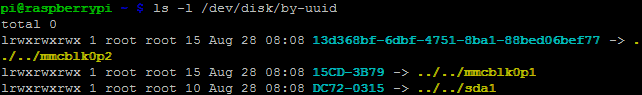
    Copy the light blue letters and numbers of the last entry (Should have something like -> ../../sda1 at the end of it).
  6. Now let’s add your drive into the fstab file so it is booted with the correct permissions.
    sudo nano /etc/fstab
  7. Now add the following line to the bottom of the file, updating uid, guid and the UUID with the values we got above. (The following should all be on a single line)
    UUID=DC72-0315 /media/ownclouddrive auto uid=33,gid=33,umask=0027,dmask=0027, noatime 0 0
  8. Reboot the Raspberry Pi and the drives should automatically be mounted. If they are mounted we’re all good to go.

Basic First Setup

I will briefly go through the basics of setting up Owncloud Raspberry Pi here. If you want more information I highly recommend checkout out the manuals on their website, you can find them here.
  1. In your browser enter your Pi’s IP address in my case it is 192.168.1.116.
  2. Once you go to the IP you’re like to get a certificate error, simply add this to your exception list as it will be safe to proceed.
  3. When you first open up ownCloud you should be presented with a simple setup screen and no errors.
  4. Enter your desired username and password.
  5. Click on storage & database and enter your external drive /media/ownclouddrive (Skip this step if you didn’t setup an external drive).
  6. Click finish setup.

2015年12月6日

Connecting to MSSQL from Fedora (and then Python 2.7)

source: http://blog.mdda.net/oss/2015/02/11/mssql-from-fedora-with-python/

With a heavy heart, I find myself having to talk to an MSSQL database. Fortunately, I can do this from a Linux (Fedora) VPS, so all is not lost.
For the following write-up (which are really just notes to myself), these links were helpful :

Step 1 : Check there’s no firewall in the way

Try the port to check that the response differs from one with no server sitting on it :
telnet 192.168.x.y 1433

Step 2 : Install FreeTDS

The FreeTDS package is the one that Fedora uses :
yum install freetds freetds-devel unixODBC unixODBC-devel

Step 3 : Check that simple queries run (command line - direct)

Using the tsql utility (from FreeTDS), test that the basic connection works (each SQL command needs to be followed by ‘go’ on a separate line to get it to execute) :
tsql -H hostname.of.the.server -p 1433 -U username-for-db
#(enter password here not on command line to avoid it appearing in history, or in process list)
When the tsql prompt comes up,
# Do a fully-qualified query 
select count(*) from DATABASENAME.dbo.TABLENAME

# Do the same, drilled down
use DATABASENAME
select count(*) from TABLENAME

# Get a listing of the tables available
SELECT * FROM information_schema.tables where TABLE_TYPE = 'BASE TABLE'

Step 4 : Check that simple queries run (command line - named server)

In order to connect to the database by ‘name’, add it as an entry into /etc/freetds.conf :
[arbitrary-tds-server-title]
  host = hostname.of.the.server
  port = 1433
  tds version = 7.0
Then queries can be run using the given name (which will then be able to pick out the appropriate hostname and port from the configuration file) :
tsql -S arbitrary-tds-server-title -U username-for-db
#(enter password, not-in-history)

Step 5 : Set up ODBC configurations

Firstly, find the driver locations (on disk!) to put into /etc/odbcinst.ini :
find / -iname 'libtds*.so'
Then, create a suitable entry in /etc/odbcinst.ini, so that ODBC know to talk to the FreeTDS drivers :
[FreeTDS]
Description = MS SQL database access with Free TDS
Driver64    = /usr/lib64/libtdsodbc.so
Setup64     = /usr/lib64/libtdsS.so
FileUsage   = 1
Then, create an entry in /etc/odbc.ini (which may have to be created) :
[sqlserverdatasource-name-is-arbitrary]
Driver      = FreeTDS
Description = ODBC connection via FreeTDS
Trace       = No
Servername  = arbitrary-tds-server-title
#Database    = <name of your database - may be useful to restrict usage>

Step 6 : Set up Python connection to ODBC

yum install pyodbc
And then one can use it in the Python shell :
python
>>> import pyodbc
>>> dsn='sqlserverdatasource-name-is-arbitrary'
>>> user='username-for-db'
>>> password='XXXXXXXX'
>>> database='DATABASENAME'
>>> con_string='DSN=%s;UID=%s;PWD=%s;DATABASE=%s;' % (dsn, user, password, database)
>>> cnxn = pyodbc.connect(con_string)
>>> cursor = cnxn.cursor()
>>> cursor.execute("select count(*) from TABLENAME")
<pyodbc.Cursor object at 0x7fe4fd2a0b10>
>>> row=cursor.fetchone()
>>> row
(249619, )

Step 7 : Read up on ODBC databases in Python

For more, see the PyODBC getting started guide.

https://azure.microsoft.com/en-us/documentation/articles/sql-database-develop-python-simple-windows/

This topic presents a code sample written in Python. The sample runs on a Windows computer. The sample and connects to Azure SQL Database by using the pymssql driver.

Requirements

Install the required modules

Install pymssql.
Make sure you choose the correct whl file.
For example : If you are using Python 2.7 on a 64 bit machine choose : pymssql‑2.1.1‑cp27‑none‑win_amd64.whl. Once you download the .whl file place it in the the C:/Python27 folder.
Now install the pymssql driver using pip from command line. cd into C:/Python27 and run the following
pip install pymssql2.1.1cp27nonewin_amd64.whl
Instructions to enable the use pip can be found here

Create a database and retrieve your connection string

See the Getting Started Topic to learn how to create a sample database and retrieve your connection string. It is important you follow the guide to create an AdventureWorks database template. The samples shown below only work with the AdventureWorks schema.

Connect to your SQL Database

The pymssql.connect function is used to connect to SQL Database.
import pymssql
conn = pymssql.connect(server='yourserver.database.windows.net', user='yourusername@yourserver', password='yourpassword', database='AdventureWorks')

Execute an SQL SELECT statement

The cursor.execute function can be used to retrieve a result set from a query against SQL Database. This function essentially accepts any query and returns a result set which can be iterated over with the use of cursor.fetchone().
import pymssql
conn = pymssql.connect(server='yourserver.database.windows.net', user='yourusername@yourserver', password='yourpassword', database='AdventureWorks')
cursor = conn.cursor()
cursor.execute('SELECT c.CustomerID, c.CompanyName,COUNT(soh.SalesOrderID) AS OrderCount FROM SalesLT.Customer AS c LEFT OUTER JOIN SalesLT.SalesOrderHeader AS soh ON c.CustomerID = soh.CustomerID GROUP BY c.CustomerID, c.CompanyName ORDER BY OrderCount DESC;')
row = cursor.fetchone()
while row:
    print str(row[0]) + " " + str(row[1]) + " " + str(row[2])   
    row = cursor.fetchone()

Insert a row, pass parameters, and retrieve the generated primary key

In SQL Database the IDENTITY property and the SEQUENCE object can be used to auto-generate primary key values.
import pymssql
conn = pymssql.connect(server='yourserver.database.windows.net', user='yourusername@yourserver', password='yourpassword', database='AdventureWorks')
cursor = conn.cursor()
cursor.execute("INSERT SalesLT.Product (Name, ProductNumber, StandardCost, ListPrice, SellStartDate) OUTPUT INSERTED.ProductID VALUES ('SQL Server Express', 'SQLEXPRESS', 0, 0, CURRENT_TIMESTAMP)")
row = cursor.fetchone()
while row:
    print "Inserted Product ID : " +str(row[0])
    row = cursor.fetchone()

Transactions

This code example demonstrates the use of transactions in which you:
-Begin a transaction
-Insert a row of data
-Rollback your transaction to undo the insert
import pymssql
conn = pymssql.connect(server='yourserver.database.windows.net', user='yourusername@yourserver', password='yourpassword', database='AdventureWorks')
cursor = conn.cursor()
cursor.execute("BEGIN TRANSACTION")
cursor.execute("INSERT SalesLT.Product (Name, ProductNumber, StandardCost, ListPrice, SellStartDate) OUTPUT INSERTED.ProductID VALUES ('SQL Server Express New', 'SQLEXPRESS New', 0, 0, CURRENT_TIMESTAMP)")
cnxn.rollback()

Next steps

For more information, see the Python Developer Center.

Example to Read/Write Excel for Python 3.5


$ pip install openpyxl
$ pip install pillow
 

Write Sample code:

from openpyxl import Workbook
wb = Workbook()

# grab the active worksheet
ws = wb.active

# Data can be assigned directly to cells
ws['A1'] = 42

# Rows can also be appended
ws.append([1, 2, 3])

# Python types will automatically be converted
import datetime
ws['A2'] = datetime.datetime.now()

# Save the file
wb.save("sample.xlsx")
 

Read Sample code:

 
from xlrd import open_workbook

book = open_workbook('simple.xls',on_demand=True)
for name in book.sheet_names():
    if name.endswith('2'):
        sheet = book.sheet_by_name(name)

        # Attempt to find a matching row (search the first column for 'john')
        rowIndex = -1
        for cell in sheet.col(0): # 
            if 'john' in cell.value:
                break

        # If we found the row, print it
        if row != -1:
            cells = sheet.row(row)
            for cell in cells:
                print cell.value

        book.unload_sheet(name) 

The easiest way to understand xs is to show an example. I will take a data example from the pivot table article.
First we get the data uploaded into a simple pivot table. Do my standard imports, read in the data and create my pivot table:
import pandas as pd
import numpy as np

df = pd.read_excel("sales-funnel.xlsx")
table = pd.pivot_table(df,index=["Manager","Rep","Product"],
               values=["Price","Quantity"],
               aggfunc=[np.sum,np.mean],fill_value=0)
table


sum mean


Price Quantity Price Quantity
Manager Rep Product


Debra Henley Craig Booker CPU 65000 2 32500 1.0
Maintenance 5000 2 5000 2.0
Software 10000 1 10000 1.0
Daniel Hilton CPU 105000 4 52500 2.0
Software 10000 1 10000 1.0
John Smith CPU 35000 1 35000 1.0
Maintenance 5000 2 5000 2.0
Fred Anderson Cedric Moss CPU 95000 3 47500 1.5
Maintenance 5000 1 5000 1.0
Software 10000 1 10000 1.0
Wendy Yule CPU 165000 7 82500 3.5
Maintenance 7000 3 7000 3.0
Monitor 5000 2 5000 2.0
This is fairly straightforward once you understand the pivot_table syntax.
Now, let’s take a look at what xs can do:
table.xs('Debra Henley', level=0)


sum mean


Price Quantity Price Quantity
Rep Product


Craig Booker CPU 65000 2 32500 1
Maintenance 5000 2 5000 2
Software 10000 1 10000 1
Daniel Hilton CPU 105000 4 52500 2
Software 10000 1 10000 1
John Smith CPU 35000 1 35000 1
Maintenance 5000 2 5000 2
Ok, this is pretty interesting. xs allows me to drill down to one cross-section of the pivot table. We can drill down multiple levels as well. If we want to just see one rep’s results:
table.xs(('Debra Henley','Craig Booker'), level=0)

sum mean

Price Quantity Price Quantity
Product


CPU 65000 2 32500 1
Maintenance 5000 2 5000 2
Software 10000 1 10000 1
If you’re like me, you just had light bulb go off and realize that a lot of cutting and pasting you have done in Excel can be a thing of the past.
We need the get_level_values to make this work as seamlessly as possible. For example, if we want to see all the Manager values:
table.index.get_level_values(0)
Index([u'Debra Henley', u'Debra Henley', u'Debra Henley', u'Debra Henley', u'Debra Henley', u'Debra Henley', u'Debra Henley', u'Fred Anderson', u'Fred Anderson', u'Fred Anderson', u'Fred Anderson', u'Fred Anderson', u'Fred Anderson'], dtype='object')
If we want to see all the rep values:
table.index.get_level_values(1)
Index([u'Craig Booker', u'Craig Booker', u'Craig Booker', u'Daniel Hilton', u'Daniel Hilton', u'John Smith', u'John Smith', u'Cedric Moss', u'Cedric Moss', u'Cedric Moss', u'Wendy Yule', u'Wendy Yule', u'Wendy Yule'], dtype='object')
To make it a little simpler for iterating, use unique :
table.index.get_level_values(0).unique()
array([u'Debra Henley', u'Fred Anderson'], dtype=object)
Now it should be clear what we’re about to do. I’ll print it out first so you can see.
for manager in table.index.get_level_values(0).unique():
    print(table.xs(manager, level=0))
                              sum            mean
                            Price Quantity  Price Quantity
Rep           Product
Craig Booker  CPU           65000        2  32500        1
              Maintenance    5000        2   5000        2
              Software      10000        1  10000        1
Daniel Hilton CPU          105000        4  52500        2
              Software      10000        1  10000        1
John Smith    CPU           35000        1  35000        1
              Maintenance    5000        2   5000        2
                            sum            mean
                          Price Quantity  Price Quantity
Rep         Product
Cedric Moss CPU           95000        3  47500      1.5
            Maintenance    5000        1   5000      1.0
            Software      10000        1  10000      1.0
Wendy Yule  CPU          165000        7  82500      3.5
            Maintenance    7000        3   7000      3.0
            Monitor        5000        2   5000      2.0
As we pull it all together, it is super simple to create a single Excel sheet with one tab per manager:
writer = pd.ExcelWriter('output.xlsx')

for manager in table.index.get_level_values(0).unique():
    temp_df = table.xs(manager, level=0)
    temp_df.to_excel(writer,manager)

writer.save()
You now get an output that looks like this:
pivot table output

Stop and Think

As you sit back and think about this code, just take a second to revel in how much we are doing with 7 lines of code (plus 2 imports):
import pandas as pd
import numpy as np

df = pd.read_excel("sales-funnel.xlsx")
table = pd.pivot_table(df,index=["Manager","Rep","Product"], values=["Price","Quantity"],aggfunc=[np.sum,np.mean],fill_value=0)
writer = pd.ExcelWriter('output.xlsx')
for manager in table.index.get_level_values(0).unique():
    temp_df = table.xs(manager, level=0)
    temp_df.to_excel(writer,manager)
writer.save()
We have just read in an Excel file, created a powerful summary of data, then broken the data up into an output Excel file with separate tabs for each manager. Just by using 9 lines of code!
I think my excitement about this functionality is warranted.

Taking It One Step Further

In some cases, you might want to generate separate files per manager or do some other manipulation. It should be pretty simple to understand how to do so given the examples above.
To close out this discussion, I decided I would wrap things up with a fully functional program that utilizes additional python functions to make this script a truly useful program that utilizes good python programming practices so that you can scale it up for your own needs:
"""
Sample report generation script from pbpython.com

This program takes an input Excel file, reads it and turns it into a
pivot table.

The output is saved in multiple tabs in a new Excel file.
"""

import argparse
import pandas as pd
import numpy as np


def create_pivot(infile, index_list=["Manager", "Rep", "Product"],
                 value_list=["Price", "Quantity"]):
    """
    Read in the Excel file, create a pivot table and return it as a DataFrame
    """
    df = pd.read_excel(infile)
    table = pd.pivot_table(df, index=index_list,
                           values=value_list,
                           aggfunc=[np.sum, np.mean], fill_value=0)
    return table


def save_report(report, outfile):
    """
    Take a report and save it to a single Excel file
    """
    writer = pd.ExcelWriter(outfile)
    for manager in report.index.get_level_values(0).unique():
        temp_df = report.xs(manager, level=0)
        temp_df.to_excel(writer, manager)
    writer.save()

if __name__ == "__main__":
    parser = argparse.ArgumentParser(description='Script to generate sales report')
    parser.add_argument('infile', type=argparse.FileType('r'),
                        help="report source file in Excel")
    parser.add_argument('outfile', type=argparse.FileType('w'),
                        help="output file in Excel")
    args = parser.parse_args()
    # We need to pass the full file name instead of the file object
    sales_report = create_pivot(args.infile.name)
    save_report(sales_report, args.outfile.name)


The simplest example of reading a CSV file:
import csv
with open('some.csv', newline='') as f:
    reader = csv.reader(f)
    for row in reader:
        print(row)
Reading a file with an alternate format:
import csv
with open('passwd', newline='') as f:
    reader = csv.reader(f, delimiter=':', quoting=csv.QUOTE_NONE)
    for row in reader:
        print(row)
The corresponding simplest possible writing example is:
import csv
with open('some.csv', 'w', newline='') as f:
    writer = csv.writer(f)
    writer.writerows(someiterable)
Since open() is used to open a CSV file for reading, the file will by default be decoded into unicode using the system default encoding (see locale.getpreferredencoding()). To decode a file using a different encoding, use the encoding argument of open:
import csv
with open('some.csv', newline='', encoding='utf-8') as f:
    reader = csv.reader(f)
    for row in reader:
        print(row)
The same applies to writing in something other than the system default encoding: specify the encoding argument when opening the output file.
Registering a new dialect:
import csv
csv.register_dialect('unixpwd', delimiter=':', quoting=csv.QUOTE_NONE)
with open('passwd', newline='') as f:
    reader = csv.reader(f, 'unixpwd')
A slightly more advanced use of the reader — catching and reporting errors:
import csv, sys
filename = 'some.csv'
with open(filename, newline='') as f:
    reader = csv.reader(f)
    try:
        for row in reader:
            print(row)
    except csv.Error as e:
        sys.exit('file {}, line {}: {}'.format(filename, reader.line_num, e))
And while the module doesn’t directly support parsing strings, it can easily be done:
import csv
for row in csv.reader(['one,two,three']):
    print(row)
Footnotes
[1](1, 2) If newline='' is not specified, newlines embedded inside quoted fields will not be interpreted correctly, and on platforms that use \r\n linendings on write an extra \r will be added. It should always be safe to specify newline='', since the csv module does its own (universal) newline handling.

2015年11月25日

How to setup Python 3.4 to access MS SQL

http://pymssql.org/en/latest/intro.html

Getting started

Generally, you will want to install pymssql with:
pip install pymssql
FreeTDS is required. On some platforms, we provide a pre-compiled FreeTDS to make installing easier, but you may want to install FreeTDS before doing pip install pymssql if you run into problems or need features or bug fixes in a newer version of FreeTDS. You can build FreeTDS from source if you want the latest. If you’re okay with the latest version that your package manager provides, then you can use your package manager of choice to install FreeTDS. E.g.:
  • Ubuntu/Debian:
    sudo apt-get install freetds-dev
    
  • Mac OS X with Homebrew:
    brew install freetds
    

Docker

(Experimental)
Another possible way to get started quickly with pymssql is to use a Docker image.
See the Docker docs for installation instructions for a number of platforms; you can try this link: https://docs.docker.com/installation/#installation
There is a pymssql docker image on the Docker Registry at:
https://registry.hub.docker.com/u/pymssql/pymssql/
It is a Docker image with:
  • Ubuntu 14.04 LTS (trusty)
  • Python 2.7.6
  • pymssql 2.1.2.dev
  • FreeTDS 0.91
  • SQLAlchemy 0.9.8
  • Alembic 0.7.4
  • Pandas 0.15.2
  • Numpy 1.9.1
  • IPython 2.3.1
To try it, first download the image (this requires Internet access and could take a while):
docker pull pymssql/pymssql
Then run a Docker container using the image with:
docker run -it --rm pymssql/pymssql
By default, if no command is specified, an IPython shell is invoked. You can override the command if you wish – e.g.:
docker run -it --rm pymssql/pymssql bin/bash
Here’s how using the Docker container looks in practice:
$ docker pull pymssql/pymssql
...
$ docker run -it --rm pymssql/pymssql
Python 2.7.6 (default, Mar 22 2014, 22:59:56)
Type "copyright", "credits" or "license" for more information.

IPython 2.1.0 -- An enhanced Interactive Python.
?         -> Introduction and overview of IPython's features.
%quickref -> Quick reference.
help      -> Python's own help system.
object?   -> Details about 'object', use 'object??' for extra details.

In [1]: import pymssql; pymssql.__version__
Out[1]: u'2.1.1'

In [2]: import sqlalchemy; sqlalchemy.__version__
Out[2]: '0.9.7'

In [3]: import pandas; pandas.__version__
Out[3]: '0.14.1'

http://pymssql.org/en/latest/_mssql_examples.html

_mssql examples

Example scripts using _mssql module.

Quickstart usage of various features

import _mssql
conn = _mssql.connect(server='SQL01', user='user', password='password', \
    database='mydatabase')
conn.execute_non_query('CREATE TABLE persons(id INT, name VARCHAR(100))')
conn.execute_non_query("INSERT INTO persons VALUES(1, 'John Doe')")
conn.execute_non_query("INSERT INTO persons VALUES(2, 'Jane Doe')")
# how to fetch rows from a table
conn.execute_query('SELECT * FROM persons WHERE salesrep=%s', 'John Doe')
for row in conn:
    print "ID=%d, Name=%s" % (row['id'], row['name'])
New in version 2.1.0: Iterating over query results by iterating over the connection object just like it’s already possible with pymssql connections is new in 2.1.0.
# examples of other query functions
numemployees = conn.execute_scalar("SELECT COUNT(*) FROM employees")
numemployees = conn.execute_scalar("SELECT COUNT(*) FROM employees WHERE name LIKE 'J%'")    # note that '%' is not a special character here
employeedata = conn.execute_row("SELECT * FROM employees WHERE id=%d", 13)
# how to fetch rows from a stored procedure
conn.execute_query('sp_spaceused')   # sp_spaceused without arguments returns 2 result sets
res1 = [ row for row in conn ]       # 1st result
res2 = [ row for row in conn ]       # 2nd result
# how to get an output parameter from a stored procedure
sqlcmd = """
DECLARE @res INT
EXEC usp_mystoredproc @res OUT
SELECT @res
"""
res = conn.execute_scalar(sqlcmd)
# how to get more output parameters from a stored procedure
sqlcmd = """
DECLARE @res1 INT, @res2 TEXT, @res3 DATETIME
EXEC usp_getEmpData %d, %s, @res1 OUT, @res2 OUT, @res3 OUT
SELECT @res1, @res2, @res3
"""
res = conn.execute_row(sqlcmd, (13, 'John Doe'))
# examples of queries with parameters
conn.execute_query('SELECT * FROM empl WHERE id=%d', 13)
conn.execute_query('SELECT * FROM empl WHERE name=%s', 'John Doe')
conn.execute_query('SELECT * FROM empl WHERE id IN (%s)', ((5, 6),))
conn.execute_query('SELECT * FROM empl WHERE name LIKE %s', 'J%')
conn.execute_query('SELECT * FROM empl WHERE name=%(name)s AND city=%(city)s', \
    { 'name': 'John Doe', 'city': 'Nowhere' } )
conn.execute_query('SELECT * FROM cust WHERE salesrep=%s AND id IN (%s)', \
    ('John Doe', (1, 2, 3)))
conn.execute_query('SELECT * FROM empl WHERE id IN (%s)', (tuple(xrange(4)),))
conn.execute_query('SELECT * FROM empl WHERE id IN (%s)', \
    (tuple([3, 5, 7, 11]),))
conn.close()
Please note the usage of iterators and ability to access results by column name. Also please note that parameters to connect method have different names than in pymssql module.

An example of exception handling

import _mssql

conn = _mssql.connect(server='SQL01', user='user', password='password',
                      database='mydatabase')
try:
    conn.execute_non_query('CREATE TABLE t1(id INT, name VARCHAR(50))')
except _mssql.MssqlDatabaseException as e:
    if e.number == 2714 and e.severity == 16:
        # table already existed, so quieten the error
    else:
        raise # re-raise real error
finally:
    conn.close()

Custom message handlers

New in version 2.1.1.
You can provide your own message handler callback function that will be invoked by the stack with informative messages sent by the server. Set it on a per _mssql connection basis by using the _mssql.MSSQLConnection.set_msghandler() method:
import _mssql

def my_msg_handler(msgstate, severity, srvname, procname, line, msgtext):
    """
    Our custom handler -- It simpy prints a string to stdout assembled from
    the pieces of information sent by the server.
    """
    print("my_msg_handler: msgstate = %d, severity = %d, procname = '%s', "
          "line = %d, msgtext = '%s'" % (msgstate, severity, procname,
                                         line, msgtext))

conn = _mssql.connect(server='SQL01', user='user', password='password')
try:
    conn.set_msghandler(my_msg_handler)  # Install our custom handler
    cnx.execute_non_query("USE mydatabase")  # It gets called at this point
finally:
    conn.close()

2015年11月22日

python 3.4 Error - No module named 'PIL'

Error to install :  from PIL import Image, ImageTk
Error message:  ImportError: No module named 'PIL'

Solution: pip install pillow


More info about PIL at http://effbot.org/imagingbook/introduction.htm

Python is a good tool for stock price analysis

Source Info: http://pythonprogramming.net/advanced-matplotlib-graphing-charting-tutorial/

Advanced Matplotlib Series (videos and ending source only)


Once you have a basic understanding of how Matplotlib works, you might have an interest in taking your knowledge a bit further. Some of the most complex graphing needs come in the form of stock analysis and charting, or Forex. In this tutorial series, we're going to cover where and how to automatically grab, sort, and organize some free stock and forex pricing data. Next, we're going to chart it using some of the more popular indicators as an example. Here, we'll do MACD (Moving Average Convergence Divergence) and the RSI (Relative Strength Index). To help us calculate these, we will use NumPy, but otherwise we will calculate these all on our own.
To acquire the data, we're going to use the Yahoo finance API. This API returns historical price data for the ticker symbol we specify and for the time length we ask for. The larger the time frame, the lower the resolution of data we get. So, if you ask for a 1-day time frame for AAPL, you will get 3-minute OHLC (open high low close) data. If you ask for 10 years worth, you will get daily data, or even 3 day time frames. Keep this in mind and choose a time frame that fits your goals. Also, if you choose a low enough time frame and get high enough granularity, the API will return the time in a unix time stamp, as compared to a date stamp.
Once we have the data, we will want to graph it. To start, we'll just plot the lines, but most people will want to plot a candlestick instead. We will use Matplotlib's candlestick function, and make a simple edit to it to improve it slightly. On this same chart, we'll also overlay a few moving average calculations.
After this, we're going to create a subplot, and graph the volume. We cannot plot volume on the same subplot immediately, because the scale is different. To start, we will plot the volume underneath in another sub plot, but eventually we'll actually overlay volume on the same figure and make it somewhat transparent.
Then, we're going to add 2 sub plots and plot an RSI indicator on top and the MACD indicator on the bottom. For all of these, we're going to share the X axis, so we can zoom in and out in 1 plot and they will all match the same time frame.
We're going to plot in date format for the X axis, and customize just about all of the things we can for aesthetics. This includes changing tick label colors, edge / spine colors, line colors, OHLC candlestick colors, learn how to create a filled graph (for volume), histograms, draw specific lines (hline for RSI), and a whole lot more.
Here's the end-result (I have both a Python 3 and a Python 2 version for this. Python 3 first, then Python 2. Make sure you're using the one that matches your Python Version!):
# THIS VERSION IS FOR PYTHON 3 #
import urllib.request, urllib.error, urllib.parse
import time
import datetime
import numpy as np
import matplotlib.pyplot as plt
import matplotlib.ticker as mticker
import matplotlib.dates as mdates
from matplotlib.finance import candlestick_ohlc
import matplotlib
import pylab
matplotlib.rcParams.update({'font.size': 9})

def rsiFunc(prices, n=14):
    deltas = np.diff(prices)
    seed = deltas[:n+1]
    up = seed[seed>=0].sum()/n
    down = -seed[seed<0].sum()/n
    rs = up/down
    rsi = np.zeros_like(prices)
    rsi[:n] = 100. - 100./(1.+rs)

    for i in range(n, len(prices)):
        delta = deltas[i-1] # cause the diff is 1 shorter

        if delta>0:
            upval = delta
            downval = 0.
        else:
            upval = 0.
            downval = -delta

        up = (up*(n-1) + upval)/n
        down = (down*(n-1) + downval)/n

        rs = up/down
        rsi[i] = 100. - 100./(1.+rs)

    return rsi

def movingaverage(values,window):
    weigths = np.repeat(1.0, window)/window
    smas = np.convolve(values, weigths, 'valid')
    return smas # as a numpy array


def ExpMovingAverage(values, window):
    weights = np.exp(np.linspace(-1., 0., window))
    weights /= weights.sum()
    a =  np.convolve(values, weights, mode='full')[:len(values)]
    a[:window] = a[window]
    return a


def computeMACD(x, slow=26, fast=12):
    """
    compute the MACD (Moving Average Convergence/Divergence) using a fast and slow exponential moving avg'
    return value is emaslow, emafast, macd which are len(x) arrays
    """
    emaslow = ExpMovingAverage(x, slow)
    emafast = ExpMovingAverage(x, fast)
    return emaslow, emafast, emafast - emaslow


def bytespdate2num(fmt, encoding='utf-8'):
    strconverter = mdates.strpdate2num(fmt)
    def bytesconverter(b):
        s = b.decode(encoding)
        return strconverter(s)
    return bytesconverter

def graphData(stock,MA1,MA2):

    '''
        Use this to dynamically pull a stock:
    '''
    try:
        print('Currently Pulling',stock)
        urlToVisit = 'http://chartapi.finance.yahoo.com/instrument/1.0/'+stock+'/chartdata;type=quote;range=10y/csv'
        stockFile =[]
        try:
            sourceCode = urllib.request.urlopen(urlToVisit).read().decode()
            splitSource = sourceCode.split('\n')
            for eachLine in splitSource:
                splitLine = eachLine.split(',')
                if len(splitLine)==6:
                    if 'values' not in eachLine:
                        stockFile.append(eachLine)
        except Exception as e:
            print(str(e), 'failed to organize pulled data.')
    except Exception as e:
        print(str(e), 'failed to pull pricing data')

    try:
        date, closep, highp, lowp, openp, volume = np.loadtxt(stockFile,delimiter=',', unpack=True,
                                                              converters={ 0: bytespdate2num('%Y%m%d')})
        x = 0
        y = len(date)
        newAr = []
        while x < y:
            appendLine = date[x],openp[x],highp[x],lowp[x],closep[x],volume[x]
            newAr.append(appendLine)
            x+=1
            
        Av1 = movingaverage(closep, MA1)
        Av2 = movingaverage(closep, MA2)

        SP = len(date[MA2-1:])
            
        fig = plt.figure(facecolor='#07000d')

        ax1 = plt.subplot2grid((6,4), (1,0), rowspan=4, colspan=4, axisbg='#07000d')
        candlestick_ohlc(ax1, newAr[-SP:], width=.6, colorup='#53c156', colordown='#ff1717')

        Label1 = str(MA1)+' SMA'
        Label2 = str(MA2)+' SMA'

        ax1.plot(date[-SP:],Av1[-SP:],'#e1edf9',label=Label1, linewidth=1.5)
        ax1.plot(date[-SP:],Av2[-SP:],'#4ee6fd',label=Label2, linewidth=1.5)
        
        ax1.grid(True, color='w')
        ax1.xaxis.set_major_locator(mticker.MaxNLocator(10))
        ax1.xaxis.set_major_formatter(mdates.DateFormatter('%Y-%m-%d'))
        ax1.yaxis.label.set_color("w")
        ax1.spines['bottom'].set_color("#5998ff")
        ax1.spines['top'].set_color("#5998ff")
        ax1.spines['left'].set_color("#5998ff")
        ax1.spines['right'].set_color("#5998ff")
        ax1.tick_params(axis='y', colors='w')
        plt.gca().yaxis.set_major_locator(mticker.MaxNLocator(prune='upper'))
        ax1.tick_params(axis='x', colors='w')
        plt.ylabel('Stock price and Volume')

        maLeg = plt.legend(loc=9, ncol=2, prop={'size':7},
                   fancybox=True, borderaxespad=0.)
        maLeg.get_frame().set_alpha(0.4)
        textEd = pylab.gca().get_legend().get_texts()
        pylab.setp(textEd[0:5], color = 'w')

        volumeMin = 0
        
        ax0 = plt.subplot2grid((6,4), (0,0), sharex=ax1, rowspan=1, colspan=4, axisbg='#07000d')
        rsi = rsiFunc(closep)
        rsiCol = '#c1f9f7'
        posCol = '#386d13'
        negCol = '#8f2020'
        
        ax0.plot(date[-SP:], rsi[-SP:], rsiCol, linewidth=1.5)
        ax0.axhline(70, color=negCol)
        ax0.axhline(30, color=posCol)
        ax0.fill_between(date[-SP:], rsi[-SP:], 70, where=(rsi[-SP:]>=70), facecolor=negCol, edgecolor=negCol, alpha=0.5)
        ax0.fill_between(date[-SP:], rsi[-SP:], 30, where=(rsi[-SP:]<=30), facecolor=posCol, edgecolor=posCol, alpha=0.5)
        ax0.set_yticks([30,70])
        ax0.yaxis.label.set_color("w")
        ax0.spines['bottom'].set_color("#5998ff")
        ax0.spines['top'].set_color("#5998ff")
        ax0.spines['left'].set_color("#5998ff")
        ax0.spines['right'].set_color("#5998ff")
        ax0.tick_params(axis='y', colors='w')
        ax0.tick_params(axis='x', colors='w')
        plt.ylabel('RSI')

        ax1v = ax1.twinx()
        ax1v.fill_between(date[-SP:],volumeMin, volume[-SP:], facecolor='#00ffe8', alpha=.4)
        ax1v.axes.yaxis.set_ticklabels([])
        ax1v.grid(False)
        ###Edit this to 3, so it's a bit larger
        ax1v.set_ylim(0, 3*volume.max())
        ax1v.spines['bottom'].set_color("#5998ff")
        ax1v.spines['top'].set_color("#5998ff")
        ax1v.spines['left'].set_color("#5998ff")
        ax1v.spines['right'].set_color("#5998ff")
        ax1v.tick_params(axis='x', colors='w')
        ax1v.tick_params(axis='y', colors='w')
        ax2 = plt.subplot2grid((6,4), (5,0), sharex=ax1, rowspan=1, colspan=4, axisbg='#07000d')
        fillcolor = '#00ffe8'
        nslow = 26
        nfast = 12
        nema = 9
        emaslow, emafast, macd = computeMACD(closep)
        ema9 = ExpMovingAverage(macd, nema)
        ax2.plot(date[-SP:], macd[-SP:], color='#4ee6fd', lw=2)
        ax2.plot(date[-SP:], ema9[-SP:], color='#e1edf9', lw=1)
        ax2.fill_between(date[-SP:], macd[-SP:]-ema9[-SP:], 0, alpha=0.5, facecolor=fillcolor, edgecolor=fillcolor)

        plt.gca().yaxis.set_major_locator(mticker.MaxNLocator(prune='upper'))
        ax2.spines['bottom'].set_color("#5998ff")
        ax2.spines['top'].set_color("#5998ff")
        ax2.spines['left'].set_color("#5998ff")
        ax2.spines['right'].set_color("#5998ff")
        ax2.tick_params(axis='x', colors='w')
        ax2.tick_params(axis='y', colors='w')
        plt.ylabel('MACD', color='w')
        ax2.yaxis.set_major_locator(mticker.MaxNLocator(nbins=5, prune='upper'))
        for label in ax2.xaxis.get_ticklabels():
            label.set_rotation(45)

        plt.suptitle(stock.upper(),color='w')
        plt.setp(ax0.get_xticklabels(), visible=False)
        plt.setp(ax1.get_xticklabels(), visible=False)
        
        ax1.annotate('Big news!',(date[510],Av1[510]),
            xytext=(0.8, 0.9), textcoords='axes fraction',
            arrowprops=dict(facecolor='white', shrink=0.05),
            fontsize=14, color = 'w',
            horizontalalignment='right', verticalalignment='bottom')

        plt.subplots_adjust(left=.09, bottom=.14, right=.94, top=.95, wspace=.20, hspace=0)
        plt.show()
        fig.savefig('example.png',facecolor=fig.get_facecolor())
           
    except Exception as e:
        print('main loop',str(e))

while True:
    stock = input('Stock to plot: ')
    graphData(stock,10,50)

# THIS VERSION IS FOR PYTHON 2 #
import urllib2
import time
import datetime
import numpy as np
import matplotlib.pyplot as plt
import matplotlib.ticker as mticker
import matplotlib.dates as mdates
from matplotlib.finance import candlestick
import matplotlib
import pylab
matplotlib.rcParams.update({'font.size': 9})

eachStock = 'EBAY','TSLA','AAPL'

def rsiFunc(prices, n=14):
    deltas = np.diff(prices)
    seed = deltas[:n+1]
    up = seed[seed>=0].sum()/n
    down = -seed[seed<0].sum()/n
    rs = up/down
    rsi = np.zeros_like(prices)
    rsi[:n] = 100. - 100./(1.+rs)

    for i in range(n, len(prices)):
        delta = deltas[i-1] # cause the diff is 1 shorter

        if delta>0:
            upval = delta
            downval = 0.
        else:
            upval = 0.
            downval = -delta

        up = (up*(n-1) + upval)/n
        down = (down*(n-1) + downval)/n

        rs = up/down
        rsi[i] = 100. - 100./(1.+rs)

    return rsi

def movingaverage(values,window):
    weigths = np.repeat(1.0, window)/window
    smas = np.convolve(values, weigths, 'valid')
    return smas # as a numpy array

def ExpMovingAverage(values, window):
    weights = np.exp(np.linspace(-1., 0., window))
    weights /= weights.sum()
    a =  np.convolve(values, weights, mode='full')[:len(values)]
    a[:window] = a[window]
    return a


def computeMACD(x, slow=26, fast=12):
    """
    compute the MACD (Moving Average Convergence/Divergence) using a fast and slow exponential moving avg'
    return value is emaslow, emafast, macd which are len(x) arrays
    """
    emaslow = ExpMovingAverage(x, slow)
    emafast = ExpMovingAverage(x, fast)
    return emaslow, emafast, emafast - emaslow

def graphData(stock,MA1,MA2):
    '''
        Use this to dynamically pull a stock:
    '''
    try:
        print 'Currently Pulling',stock
        print str(datetime.datetime.fromtimestamp(int(time.time())).strftime('%Y-%m-%d %H:%M:%S'))
        urlToVisit = 'http://chartapi.finance.yahoo.com/instrument/1.0/'+stock+'/chartdata;type=quote;range=10y/csv'
        stockFile =[]
        try:
            sourceCode = urllib2.urlopen(urlToVisit).read()
            splitSource = sourceCode.split('\n')
            for eachLine in splitSource:
                splitLine = eachLine.split(',')
                if len(splitLine)==6:
                    if 'values' not in eachLine:
                        stockFile.append(eachLine)
        except Exception, e:
            print str(e), 'failed to organize pulled data.'
    except Exception,e:
        print str(e), 'failed to pull pricing data'
    try:   
        date, closep, highp, lowp, openp, volume = np.loadtxt(stockFile,delimiter=',', unpack=True,
                                                              converters={ 0: mdates.strpdate2num('%Y%m%d')})
        x = 0
        y = len(date)
        newAr = []
        while x < y:
            appendLine = date[x],openp[x],closep[x],highp[x],lowp[x],volume[x]
            newAr.append(appendLine)
            x+=1
            
        Av1 = movingaverage(closep, MA1)
        Av2 = movingaverage(closep, MA2)

        SP = len(date[MA2-1:])
            
        fig = plt.figure(facecolor='#07000d')

        ax1 = plt.subplot2grid((6,4), (1,0), rowspan=4, colspan=4, axisbg='#07000d')
        candlestick(ax1, newAr[-SP:], width=.6, colorup='#53c156', colordown='#ff1717')

        Label1 = str(MA1)+' SMA'
        Label2 = str(MA2)+' SMA'

        ax1.plot(date[-SP:],Av1[-SP:],'#e1edf9',label=Label1, linewidth=1.5)
        ax1.plot(date[-SP:],Av2[-SP:],'#4ee6fd',label=Label2, linewidth=1.5)
        
        ax1.grid(True, color='w')
        ax1.xaxis.set_major_locator(mticker.MaxNLocator(10))
        ax1.xaxis.set_major_formatter(mdates.DateFormatter('%Y-%m-%d'))
        ax1.yaxis.label.set_color("w")
        ax1.spines['bottom'].set_color("#5998ff")
        ax1.spines['top'].set_color("#5998ff")
        ax1.spines['left'].set_color("#5998ff")
        ax1.spines['right'].set_color("#5998ff")
        ax1.tick_params(axis='y', colors='w')
        plt.gca().yaxis.set_major_locator(mticker.MaxNLocator(prune='upper'))
        ax1.tick_params(axis='x', colors='w')
        plt.ylabel('Stock price and Volume')

        maLeg = plt.legend(loc=9, ncol=2, prop={'size':7},
                   fancybox=True, borderaxespad=0.)
        maLeg.get_frame().set_alpha(0.4)
        textEd = pylab.gca().get_legend().get_texts()
        pylab.setp(textEd[0:5], color = 'w')

        volumeMin = 0
        
        ax0 = plt.subplot2grid((6,4), (0,0), sharex=ax1, rowspan=1, colspan=4, axisbg='#07000d')
        rsi = rsiFunc(closep)
        rsiCol = '#c1f9f7'
        posCol = '#386d13'
        negCol = '#8f2020'
        
        ax0.plot(date[-SP:], rsi[-SP:], rsiCol, linewidth=1.5)
        ax0.axhline(70, color=negCol)
        ax0.axhline(30, color=posCol)
        ax0.fill_between(date[-SP:], rsi[-SP:], 70, where=(rsi[-SP:]>=70), facecolor=negCol, edgecolor=negCol, alpha=0.5)
        ax0.fill_between(date[-SP:], rsi[-SP:], 30, where=(rsi[-SP:]<=30), facecolor=posCol, edgecolor=posCol, alpha=0.5)
        ax0.set_yticks([30,70])
        ax0.yaxis.label.set_color("w")
        ax0.spines['bottom'].set_color("#5998ff")
        ax0.spines['top'].set_color("#5998ff")
        ax0.spines['left'].set_color("#5998ff")
        ax0.spines['right'].set_color("#5998ff")
        ax0.tick_params(axis='y', colors='w')
        ax0.tick_params(axis='x', colors='w')
        plt.ylabel('RSI')

        ax1v = ax1.twinx()
        ax1v.fill_between(date[-SP:],volumeMin, volume[-SP:], facecolor='#00ffe8', alpha=.4)
        ax1v.axes.yaxis.set_ticklabels([])
        ax1v.grid(False)
        ###Edit this to 3, so it's a bit larger
        ax1v.set_ylim(0, 3*volume.max())
        ax1v.spines['bottom'].set_color("#5998ff")
        ax1v.spines['top'].set_color("#5998ff")
        ax1v.spines['left'].set_color("#5998ff")
        ax1v.spines['right'].set_color("#5998ff")
        ax1v.tick_params(axis='x', colors='w')
        ax1v.tick_params(axis='y', colors='w')
        ax2 = plt.subplot2grid((6,4), (5,0), sharex=ax1, rowspan=1, colspan=4, axisbg='#07000d')
        fillcolor = '#00ffe8'
        nslow = 26
        nfast = 12
        nema = 9
        emaslow, emafast, macd = computeMACD(closep)
        ema9 = ExpMovingAverage(macd, nema)
        ax2.plot(date[-SP:], macd[-SP:], color='#4ee6fd', lw=2)
        ax2.plot(date[-SP:], ema9[-SP:], color='#e1edf9', lw=1)
        ax2.fill_between(date[-SP:], macd[-SP:]-ema9[-SP:], 0, alpha=0.5, facecolor=fillcolor, edgecolor=fillcolor)

        plt.gca().yaxis.set_major_locator(mticker.MaxNLocator(prune='upper'))
        ax2.spines['bottom'].set_color("#5998ff")
        ax2.spines['top'].set_color("#5998ff")
        ax2.spines['left'].set_color("#5998ff")
        ax2.spines['right'].set_color("#5998ff")
        ax2.tick_params(axis='x', colors='w')
        ax2.tick_params(axis='y', colors='w')
        plt.ylabel('MACD', color='w')
        ax2.yaxis.set_major_locator(mticker.MaxNLocator(nbins=5, prune='upper'))
        for label in ax2.xaxis.get_ticklabels():
            label.set_rotation(45)

        plt.suptitle(stock.upper(),color='w')

        plt.setp(ax0.get_xticklabels(), visible=False)
        plt.setp(ax1.get_xticklabels(), visible=False)
        
        ax1.annotate('Big news!',(date[510],Av1[510]),
            xytext=(0.8, 0.9), textcoords='axes fraction',
            arrowprops=dict(facecolor='white', shrink=0.05),
            fontsize=14, color = 'w',
            horizontalalignment='right', verticalalignment='bottom')

        plt.subplots_adjust(left=.09, bottom=.14, right=.94, top=.95, wspace=.20, hspace=0)
        plt.show()
        fig.savefig('example.png',facecolor=fig.get_facecolor())
           
    except Exception,e:
        print 'main loop',str(e)

while True:
    stock = raw_input('Stock to plot: ')
    graphData(stock,10,50)